How To Sketch Level Sets

Graphing functions

One way to visualize functions is through their graphs. If $f(x,y)$ is a scalar-valued function of ii variables, $f: \R^2 \to \R$ (confused?), then its graph is the surface formed by the set of all the points $(x,y,z)$ where $z=f(10,y)$, i.eastward., the set up of points $(x,y,f(x,y))$. Past graphing this surface, nosotros can visualize the behavior of the function.

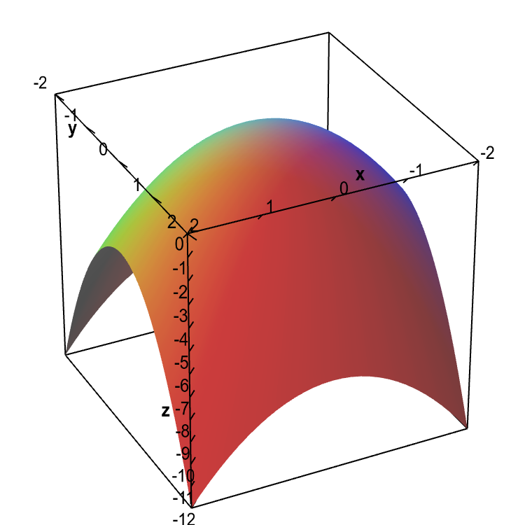
Equally an example, we graph the function $f(x,y)=-ten^two-2y^2$ using the domain divers by $-two \le 10 \le 2$ and $-2 \le y \le 2$. The graph of all points $(x,y,f(x,y))$ with $(x,y)$ in this domain is an elliptic paraboloid, every bit shown in the following effigy.

Applet loading

Graph of elliptic paraboloid. A graph of the function $f(x,y)=-ten^2-2y^two$ over the domain $-2 \le x \le 2$ and $-2 \le y \le two$.

More information near applet.

Three-dimensional plots, such every bit the in a higher place effigy, are more difficult to draw and visualize than two-dimensional plots. Moreover, the graph of a part $f(x,y,z)$ of three variables would be the set of points $(x,y,z,f(x,y,z))$ in iv dimensions, and it would be difficult to imagine what such a graph would look similar.

Another manner of visualizing a function is through level sets, i.due east., the set of points in the domain of a function where the function is constant. The nice part of of level sets is that they live in the same dimensions as the domain of the function. A level fix of a office of two variables $f(10,y)$ is a bend in the 2-dimensional $xy$-plane, called a level bend. A level fix of a function of three variables $f(x,y,z)$ is a surface in three-dimensional space, called a level surface.

Level curves

One way to collapse the graph of a scalar-valued function of ii variables into a two-dimensional plot is through level curves. A level curve of a office $f(x,y)$ is the curve of points $(x,y)$ where $f(x,y)$ is some constant value. A level bend is simply a cross section of the graph of $z=f(x,y)$ taken at a constant value, say $z=c$. A function has many level curves, as i obtains a different level bend for each value of $c$ in the range of $f(x,y)$. Nosotros can plot the level curves for a bunch of different constants $c$ together in a level curve plot, which is sometimes called a profile plot.

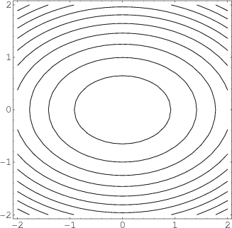
We return to the in a higher place example function $f(ten,y) = -x^2-2y^2$. For some constant $c$, the level curve $f(x,y)=c$ is the graph of $c=-x^2-2y^2$. As long every bit $c<0$, this graph is an ellipse, as 1 can rewrite the equation for the level curve every bit \brainstorm{align*} \frac{x^2}{-c} + \frac{y^2}{-c/ii} =one. \terminate{marshal*} (If $c$ is negative, then both denominators are positive.) For example, if $c=-1$, the level bend is the graph of $x^2 + 2y^2=1$. In the level curve plot of $f(10,y)$ shown below, the smallest ellipse in the eye is when $c=-1$. Working outward, the level curves are for $c=-ii, -3, \ldots, -10$.

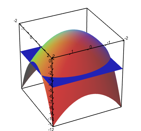
The below graph illustrates the relationship between the level curves and the graph of the function. The primal point is that a level curve $f(x,y)=c$ can exist thought of as a horizontal slice of the graph at height $z=c$. This piece is the intersection of the graph with the aeroplane $z=c$.

Applet loading

Applet loading

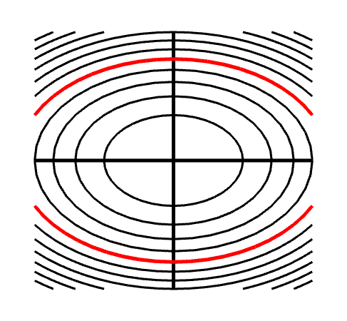
Level curves of an elliptic paraboloid shown with graph. The graph of the part $f(x,y)=-x^2-2y^2$ is shown is the kickoff panel forth with a level curve plot in the 2nd panel. The level bend $f(ten,y)=c$ is shown in cerise in the level curve plot, which is the same as the slice of the graph $z=f(x,y)$ by the plane $z=c$. Y'all can change $c$ by dragging the plane slicing the graph upwardly or down with the mouse. You lot can too change $c$ by dragging the red level curve.

More data about applet.

Topographic maps are simply level curves of the elevation of the country (or water). For instance, on standard United States Geological Survey maps, each contour line represents 10 feet of acme above sea level, as in this topographic map of Eagle Mountain, the highest mountain (well... hill) in Minnesota. The closer the contour lines are together, the steeper the slope of the land. Non surprisingly, the steepest slopes seem to exist very near the summits of Eagle Mount and Moose Mountain.

Level surfaces

For a scalar-valued functions of three variables, $f : \R^three \to \R$, we would need four dimensions to draw its graph. The graph is the set up of points $(x,y,z,f(10,y,z))$. Y'all should familiarize yourself with vectors in higher dimensions to become comfortable with the idea of four dimensions. Nonetheless, unless your heed is better at abstruse visualization than most, y'all may have a difficult time visualizing what this graph in four dimensions would look like.

Instead, nosotros tin wait at the level sets where the function is abiding. For a office of two variables, above, nosotros saw that a level ready was a curve in two dimensions that nosotros chosen a level bend. For a function of three variables, a level fix is a surface in three-dimensional space that we will call a level surface. For a abiding value $c$ in the range of $f(x,y,z)$, the level surface of $f$ is the implicit surface given by the graph of $c=f(10,y,z)$.

The below version of the level curve applet will assistance you run across that level curves and level surfaces are like concepts, equally this verion is put in the format that we volition employ for level surfaces. In this case, only i level curve $f(ten,y)=c$ is displayed at a fourth dimension.

A level curve of an elliptic paraboloid. A level bend of the part $f(ten,y) = -10^2-2y^2=c$ is shown. You can elevate the slider with the mouse to alter $c$ and hence the level curve being displayed.

More information about applet.

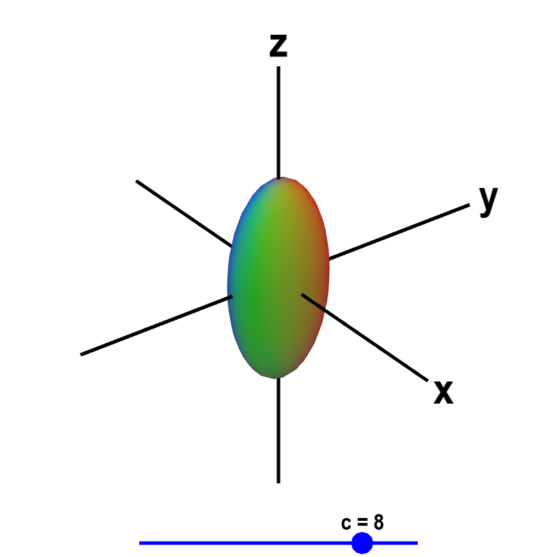
Now, nosotros wait at the function $f(x,y,z) = 10 e^{-9x^2-4y^2-z^2}$. Fifty-fifty though we can't plot the graph of $f(10,y,z)$ (without using four dimensions), we can still visualize the behavior of the part by plotting its level surfaces. We simply plot $f(10,y,z)=c$ for $c$ between 0 and x. (Note that $f(x,y,z)$ always lies betwixt $0$ and $10$. The argument of the exponential is ever negative or zero, so the value of the exponential is e'er between naught and one.) The behavior of these level surfaces is illustrated in the following applet.

Applet loading

Level surface of a function of iii variables. A level surface $f(x,y,z) = 10 e^{-9x^2-4y^two-z^2}=c$ is shown. You lot can elevate the blue point on the slider with the mouse to change $c$, and hence the level surface existence displayed.

More information nearly applet.

The significance of the level surfaces may become clearer if you think of $f(x,y,z)$ every bit giving the temperature at the betoken $(x,y,z)$. Then, the level surface $f(10,y,z)=ii$ is the surface of points where the temperature is 2. In this example, the temperature at the origin is 10 and every other point has a lower temperature. Hence, the level surface $f(10,y,z)=c$ shrinks to a indicate effectually the origin as $c$ increases to x.

As one moves away from the origin, the temperature decreases. The temperature decreases toward nix as you get far from the origin. The level surface $f(x,y,z)=0$ doesn't exist considering $f(x,y,z)$ never reaches zero. Only, if $c$ is a small-scale positive number, the level surface $f(x,y,z)=c$ is a large ellipsoid. Y'all tin can look at a couple more than examples.

Source: https://mathinsight.org/level_sets

Share this post